Digital Audio Synthesis for Dummies: Part 1

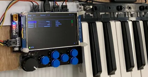
A while back I worked on a lil’ MIDI keyboard project and learnt a lot regarding digital audio signal processing. This post is the first in a series of posts related to that project and aims to provide a springboard for those who wish to get their feet wet with audio processing.

Dealing with Data 📈

When processing data of any form, we are concerned with the data’s quality. Higher quality data may lead to a more thorough analysis and better user experience, but also demand higher memory and computing requirements.

With audio, we are concerned with two dimensions of quality: sampling (time) and quantisation (bit depth).

Sampling 🔪

Sampling refers to how much we “chop” a signal. Suppose our signal is a carrot. For a stew, we may want longer samples (sparser chops). With rice, however, it's better to go with shorter samples (denser chops).

^{Blue line: original, continuous signal. Red dots: sampled, discrete signal. At higher sample rates, we chop densely, and more information is retained. At lower sample rates, we chop sparsely, but the sampled signal struggles to capture the peaks and troughs.}

Digital audio signals are represented discretely by storing samples at regular intervals instead of using a single continuous line.

The sample rate refers to how fast we chop, how fast we sample our audio. Choosing an appropriate sample rate for your application is an important consideration. A higher rate yields more information per second, at the expense of space.

Audio is usually sampled at 44.1kHz or 48kHz (i.e. 44,100 or 48,000 samples per second). But why are these rates so common? To answer this, we first need to learn about the…

Nyquist-Shannon Sampling Theorem

The Nyquist-Shannon Sampling Theorem (aka the Nyquist Theorem) is an important consideration when choosing a sample rate for your application. According to this theorem, in order to accurately reconstruct a continuous signal such as audio, it must be sampled at a rate that is at least twice the highest frequency component of the signal. This threshold is also called the Nyquist frequency.

For example, if we want to store a 1kHz audio signal, we would need to sample at 2kHz or more. Humans can hear frequencies in the range 20Hz – 20kHz, so if we want to capture all audible sounds, our sample rate needs to be at least 40kHz.

This is important to avoid aliasing, which occurs when high frequency components of a signal are mistakenly interpreted as lower frequency components. Aliasing results in distortion and can lead to inaccurate representation of the original signal.

The diagram below demonstrates aliasing, which happens when our sample rate is too low.

^{(a) Sampling a 20kHz signal at 40kHz captures the original signal correctly. (b) Sampling the same 20kHz signal at 30kHz captures an aliased (low frequency ghost) signal. (Source: Embedded Media Processing.1)}

Quantisation 🪜

While sampling deals with resolution in time, quantisation deals with resolution in dynamics (or loudness). Here, we’re concerned with two things: quality and data storage (in files or RAM).

1. Like sampling, quantisation affects how well a signal is represented. If we quantise with 1 bit, then each sample has only two possible values (0 or 1). This means we can represent square waves (where high=1, low=0). But we can’t represent sine waves since the values in between that make up a sine wave aren’t in our vocabulary.

   

   ^{Blue: original signal; Red: quantised signal. Higher quantisation leads to better audio quality. With 1 or 2 bits, we can barely tell the signal is reproduced. With more bits, the signal is more faithfully reproduced.}

   Higher quantisation also gives us greater dynamic resolution. With 1 bit, we're limited to absolute silence (0) or an ear-shattering loudness (1). With 8 bits, we have $2^8 = 256$ different "volume settings" to choose from—much more quality than simple 1s and 0s!

2. Regarding data storage, the less number of bits needed per sample, the more memory saved. When storing samples in files, most applications quantise to 16-bit integers, which allow for a decent resolution of -32,768 to +32,767 at two bytes per sample (1 byte being 8 bits). 32-bit floats are another common representation, bringing substantially greater detail at the expense of twice the space.⁴

   

   ^{Each block is an audio sample. Lower quantisation leads to more compact storage.5}

   Now when storing audio in RAM for audio processing, it's easier to work with floats in the range of -1.0 to 1.0. Why the smaller range? Well, if we work directly with the maxima, we may easily encounter errors. With integers, we would experience integer overflow, which wraps positive values to negative values—a horrid nightmare! With floats, we would venture into the territory of infinity, which disrupts subsequent computations.

   Thus, we use a smaller range to allow room for processing.

Audio Mishaps and Bugs 🐞

If you know the enemy and know yourself, you need not fear the result of a hundred battles. – Sun Tzu, The Art of War

Sometimes when experimenting with audio, something goes amiss. The most common issues are aliasing, clipping, and clicks. These pesky lil' issues may crop up when processing audio... all the more important to understand how to mitigate them.

Aliasing

We mentioned aliasing earlier. Aliasing occurs when a signal is sampled insufficiently, causing it to appear at a lower frequency.

Generally, increasing the sample rate helps (or lowering the maximum frequency). In any case, it's wise to be vigilant with your sample rate and frequency range.

Clipping ✂️

Clipping occurs when our samples go out-of-bounds, past the maximum/minimum quantisation value. Clipping may cause our signal to wraparound or flatten at the peaks and troughs.

^{Example of wraparound clipping, typically due to integer overflow/underflow.}

^{Example of a signal flattened at the peaks and troughs due to clamping.}

Clipping arises from neglecting dynamic range. It can be addressed by scaling down the signal (multiplying samples by a factor below 1) or by using dynamic range compression (loud noises are dampened, soft noises are left unchanged).

Clicks

Clicks (aka pops) occur when a signal behaves discontinuously with large differences between samples. This difference forces the speaker hardware to vibrate quickly… too quickly.

^{Signal jumps from -1.0 to 1.0, causing my speaker to pop and my ear drums to bleed from utter despair.}

Clicks may arise from trimming or combining audio recordings without applying fades. In audio synthesis, mismanagement of buffers and samples may also be a factor.⁶

Recap 🔁

Audio processing is ubiquitous in daily life. In this post, we explored how digital audio works under the hood. Hopefully we communicated on the same wavelength and no aliasing occurred on your end. 😏

In the next post, we'll look at audio synthesis: the making of audio from nothing.

To recap…

• Fundamental to audio processing is the quality of audio data. This comes in two forms: sampling and quantisation.
  • Sampling refers to the discretisation and resolution of a signal in time.
    • Higher sample rate = more information per second = higher quality.
  • Quantisation refers to the bit depth, the resolution in loudness.
    • Higher bit depth = higher quality.
  • Higher quality comes with the cost of higher memory consumption.
  • To accurately reconstruct a signal, the Nyquist Theorem states the sample rate should surpass the Nyquist frequency (twice the maximum frequency of the signal).
    • Sample rates below the signal's Nyquist frequency are prone to aliasing.
• Some common issues to audio processing are aliasing, clipping, and clicks.
  • Aliasing occurs when a signal is misinterpreted to be of lower frequency.
  • Clipping occurs when samples exceed the dynamic range and are cut.
  • Clicks occur when samples contain a large difference, causing the speaker to vibrate too quickly.